Parallel KCF Tracking
A 15-618 Final Project by Ilaï Deutel and Denis Merigoux
Summary
We modified the OpenCV implementation of the KCF object tracking algorithm to use the NVIDIA GPUs of the GHC machines. Our 1.84x final speedup obtained on a fullHD video increased the number of FPS from 8.4 to 12.8.
Background
Tracking API
An object tracking algorithm takes as input a video seens as a sequence of frames, and an initial bounding box that indicates the object to track. The algorithm offers an interface consisting of two methods:
init(initial_frame,bounding_box)which sets up the algorithm data structures;update(new_frame)which updates the position of the bounding box by identifying the position of the tracked object on thenew_frame.
Key operations
The KCF algorithm (and the other tracking algorithm) use diverse statistical learning techniques to infer the new position of the tracked object. These techniques operate on matrices, which offer potential for parallelization. However, the KCF algortihm makes use of non-linear operations such as Fourier transform to compute kernels. Because the tracking algorithm sees only one frame at a time (as in a real-time use case), the parallelization axis concerns the number of pixels in a frame, which directly influences the dimensions of the matrices handled by the algorithm.
Workload decomposition
By examining the sequential implementation of the KCF tracker in OpenCV, we broke down the time spent in each phase of the algorithm. The longest and most computational-intensive phases are in bold; they involve mostly Discrete Fourier Transform and matrix multiplication.
| Phase | Subtask | Time taken |
|---|---|---|
| Detection | Extract and pre-process the patch | 3.102 ms |
| Non-compressed custom descriptors | 0.836 ms | |
| Compressed descriptors | 30.993 ms | |
| Compressed custom descritors | 13.752 ms | |
| Compress features and KRSL | 37.745 ms | |
| Merge all features | 7.548 ms | |
| Compute the gaussian kernel | 144.494 ms | |
| Compute the FFT | 15.714 ms | |
| Calculate filter response | 22.792 ms | |
| Extract maximum response | 0.959 ms | |
| Total | 277.935 ms | |
| Extracting patches | Update bounding box | 0.000 ms |
| Non-compressed descriptors | 3.198 ms | |
| Non-compressed custom descriptors | 0.831 ms | |
| Compressed descriptors | 30.909 ms | |
| Compressed custom descriptors | 13.755 ms | |
| Update training data | 12.978 ms | |
| Total | 61.196 ms | |
| Feature compression | Update projection matrix | 87.808 ms |
| Compress | 18.144 ms | |
| Merge all features | 3.684 ms | |
| Total | 108.924 ms | |
| Least Squares Regression | Initialization | 0.001 ms |
| Calculate alphas | 142.453 ms | |
| Compute FFT | 15.592 ms | |
| Add a small value | 1.930 ms | |
| New Alphaf | 6.526 ms | |
| Update RLS model | 4.539 ms | |
| Total | 169.960 ms | |
| Total time for a frame | 625.019 ms |
The values are averaged over all the 189 frames of the test video.
Approach
Framework and starting code
Because the algorithm is very complex, we chose to modify the existing sequential KCF OpenCV implementation, rather than start from scratch. The choice of the OpenCV implementation has been made for several reasons:
- the OpenCV framework is heavily optimized and the sequenial implementation of the algorithm in the framework is then a good sequential baseline;
- the framework offers high-level bindings for CUDA specifically tailored for matrices operations;
- our project is more usable as part of an OpenCV modules than if it was written using custom conventions and APIs;
- OpenCV is very popular for image processing and speeding up one of its modules could benefit other people.
Because of this choice, our work use C++ and CUDA, and targets the GHC machines to make use of the high-end NVIDIA GTX 1080. The OpenCV CUDA bindings take care of mapping most of the higher-level operations to the hardware warps.
Testing and profiling framework
Our first main task was to implement a custom profiling and correctness testing framework on top of the starting code to be able to constantly check if our parallel implementation yield exactly the same results as the baseline implementation. The profiling is done with cycle timer with average values over all frames and the correctness test checks for the coordinates of the updated bounding box after each iteration. They must be exactly the same (no approximation).
Example of output for an incorrect implementation:
=== Sequential ===
// Performance information for the 189 frames of the video, not shown here
=== Parallel ===
// Performance information for the first 4 frames of the video, not shown here
Correctness failed at frame 3
Bounding box mismatch:
* Sequential: [286 x 720 from (635, 219)]
* Parallel: [286 x 720 from (635, 221)]
We’ll now discuss how we increased performance for each one of the three most computational-intensive phases of the algorithm.
Discrete Fourier transform
The baseline implementation used a sequential implementation of the DFT. After having noticed that this was the most time-consuming operation of the algorithm, we decided to switch to cuFFT, which is a high performance DFT library maintained by NVIDIA that specifically targets their GPUs.
OpenCV provided a binding to call cufftexec but we had to modify heavily this binding for two reasons:
- the binding only offered support for
floatmatrices and notdoublematrices; - the binding did not take into account the fact that the input and output format for the complex matrices for
cuFFTis the CCE format, which is different from the full format used in the sequential implementation.
While handling double precision matrices was fairly easy, the format translation was the main stumbling block of our project. Indeed, switching from one format to the other required a significant amount of computation that decreased performance, cancelling the benefit of using cuFFT. Instead, we preferred to modify the part of the algorithm that operated on complex spectrum matrices (after forward transform and before inverse transform) to accomodate for the native output and input format of cuFFT.
Replacing sequential FFT with cuFFT with the above accommodation triggered a decrease of 20 ms of the average computing time for updating one frame, and a local 2x speedup. Indeed, the DFT was used for computing gaussian kernels in a function used in two critical phases of the algorithm.
Updating the projection matrix
The second most time-consuming phase was performing a Principal Component Analysis. The associated function performs a Singular Values Decomposition wirth some pre-processing to update the covariance matrix. First we thought that we would have to speedup the SVD to increase performance, but a careful profiling revealed that the most time-consuming subpart was, by a large factor, the update of the covariance matrix.
In this situation, using opencv gemm (Generalized Matrix Multiplication) function was sufficient to achieve a 2x local speedup. Indeed, the matrix product multiplied a matrix by its transpose, operation that is heavily optimized on GPU but not on CPU. Is is worth noting that we tried to use gemm in another context with a matrix of size (n,m) where m >> n multiplied bu another matrix of small size; but here the disparity of sizes and the data layout caused very poor performance on the GPU, and the CPU implementation was actually faster.
Another problem that arose during the optimization of this subtask was the migration of data between the CPU and the GPU. Because the algorithm still uses the CPU for most of its operations, we need to maintain data structures on the CPU and on the GPU, with occasional transfers to update at the right time. However, the transfer of a matrix takes approximately 1 ms, which can be crucial in fast operations. We during the project tried to carefully balance the benefits of GPU speedup vs. the drawback of slow GPU<->CPU transfers. Another optimization was to have fixed-size GPU data structures to have O(1) cudaMalloc calls, to avoid loosing more precious milliseconds.
All these optimizations combined triggered a gain of another 10 ms.
Compressed descriptors
Finally, we optimized a more complicated operation involving extracting matrices descriptors. The operation consists in merging the values of the 3 channels of an image for each pixel and applying some arithmetic functions on their values to extract color names from image patches. Because of the specificity of this situation, we had to use OpenCV’s binding to write our own CUDA kernel operating on OpenCV’s GpuMat. We launched the kernels with blocks of 32x32 CUDAthreads, value chosen after the experimentations of the CUDA renderer in Assignment 2.
This optimization decreased average time by another 5 ms.
Results
Metric and inputs
The main metric for our experiment is the wall-clock time used to update the bounding box for one new frame, averaged over all 189 frames of the video (except the first one, where many data structures are set up).
The input consists in a video of 189 frames showing Charlie Chaplin walking across the screen, with a 4K resolution (2160x3840).
Parallel program time breakdown
| Phase | Subtask | Time taken |
|---|---|---|
| Detection | Extract and pre-process the patch | 3.013 ms |
| Non-compressed custom descriptors | 0.801 ms | |
| Compressed descriptors | 11.132 ms | |
| Compressed custom descritors | 13.820 ms | |
| Compress features and KRSL | 37.531 ms | |
| Merge all features | 7.441 ms | |
| Compute the gaussian kernel | 33.139 ms | |
| Compute the FFT | 15.559 ms | |
| Calculate filter response | 22.445 ms | |
| Extract maximum response | 0.948 ms | |
| Total | 145.830 ms | |
| Extracting patches | Update bounding box | 0.000 ms |
| Non-compressed descriptors | 3.119 ms | |
| Non-compressed custom descriptors | 0.767 ms | |
| Compressed descriptors | 11.159 ms | |
| Compressed custom descriptors | 13.571 ms | |
| Update training data | 12.820 ms | |
| Total | 40.979 ms | |
| Feature compression | Update projection matrix | 57.125 ms |
| Compress | 17.983 ms | |
| Merge all features | 3.619 ms | |
| Total | 73.760 ms | |
| Least Squares Regression | Initialization | 0.001 ms |
| Calculate alphas | 36.834 ms | |
| Compute FFT | 15.654 ms | |
| Add a small value | 1.904 ms | |
| New Alphaf | 6.324 ms | |
| Update RLS model | 4.633 ms | |
| Total | 60.198 ms | |
| Total time for a frame | 327.326 ms |
Impact of resolution
We tried running our program with the same video at various resolutions (480p, 720p, 1080p, 1440p, 2160p) and it was confirmed that our algorithm is useful for scaling out the resolution: the bigger the matrices, the better is the benefit for using a GPU. On the contrary, scaling in yields poor performance on the GPU with data transfer times dominating the computations: sequential implementation runs faster.
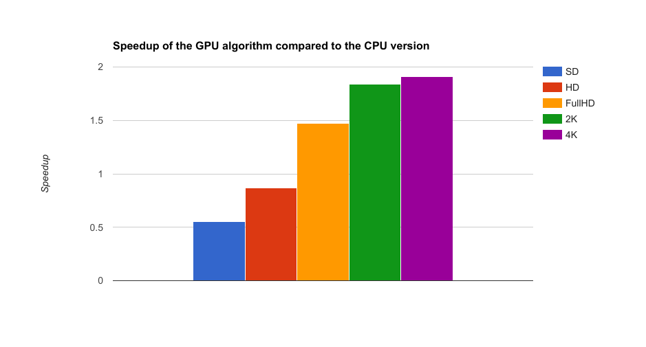
We notice that the speedup reaches asymptotycally a 2x value whith high resolutions, corresponding to the natural speedup of using the GPU for these particular tasks (transfer times are negligible).
Possible improvements
While we have optimized the most time-consuming parts of the algorithm using CUDA, a better solution would be to implement the whole algorithm using only GPU data structures and kernels. We could then achieve a 2x or 2.5x speedup on all of the little tasks that take 2 or 3 ms each, effectively increasing the overall speedup.
Conclusion
We haven’t reach our main goal of processing a fullHD video in real time with a decent framerate, but we have definitely improved significantly the performance of a popular tracking module of OpenCV, using a piece of hardware specifically adapted for image processing (GPU).